

Introduction
The models on the basis of logit- or probit-functions have more than semi-centennial history (Finney, 1947, 1971; Belenky, 1963). The development of this methodology from the usage of semi-heuristic regularities to the full regression models based on the principle of maximum likelihood increased the accuracy in the assessment of toxicometric characteristics not so much as created prerequisites for the usage of powerful and effective ways to control the impact of random factors.
In solving the problems of eco-toxicology it is impossible to carry out a “sterile” experiment with a chemically standard toxic substance. It is also difficult to assess the level of dangerous exposure in the conditions of specific, age-related and gender specificity of populations, environment heterogeneity, the influence of seasonal climatic changes and other contributing factors. The modern approach to solving these problems is associated with the usage of regression models with mixed parameters (mixed effect model – Pinheiro, Bates, 2000; Demidenko, 2013; Chetverikov, 2015). These models create prerequisites for the significant increase in the level of generalization of target results and their extension to other spatial, temporal or biological levels of arrangement. The interest to mixed models constantly grows: according to the data of Google Scholar, only in 2017 608000 articles were published, among them 17 800 articles in ecology (in Russian – not more than 3).
The essence of this method is that the effects (factors) influencing the dependent variables are conditionally divided into two types: fixed and random. Here the fixed effects are usually of interest to an investigator i.e. those independent variables, the levels of which are stated or controlled (in our case – dose of snake’s venom). For random effects it is usually difficult to compose the plan of factors levels variation, and they can take on random values among the possible ones in the entire assembly. Philosophic methodological aspects of dividing the effects on types are highly ambiguous (Gelman, 2005). Therefore, below we will interpret all the contributing factors as random ones influencing to some degree the process of intoxication and death of experimental animals (their sex, subspecies and the area of snake capture, venom color etc.).
The purpose of the work is to assess the results of using models with mixed parameters on the concrete samples of eco-toxicological data. The main tasks of the investigation: first, to show the strategy of the analysis of separate model versions and the possibility of their interpretation; second, to check the reliability and usefulness of the method used to solve some problems of toxinology. The meaningful ecological conclusions concerning the spatial distribution of distinct snake populations are outside the scope of this paper.
Materials
The samples of poisonous secret were obtained from common snakes Vipera berus (Linnaeus, 1758), captured in 12 different geographical regions (below – variable habitat) of the European part of Russia. The subspecies affiliation (variable – subspecies) of the snakes of the studied populations – V.b. berus (Linnaeus, 1758) and V. b. nikolskii (Vedmederija et al., 1986) was stated according to their morphological signs and venom color (Bakiev et al., 2005; Milto, Zinenko, 2005). The division into two subspecies should be considered as conditional, as the part of the populations dwells in the zone of intergradations of these subspecies and have mixed signs. So, in Penza district of Penza Region the population, in which one part of snakes has yellow venom (sample 8) characteristic for the nominative form of V.b. berus, while the other part – colorless venom (sample 7) characteristic for the forest-steppe form V.b. nikolskii.
The preparations of poisonous secret were administered intraperitoneally to white laboratory mice, males and females (variable – sex) weighing 20±1.0 г. For each venom specimen of adders captured in different regions, 5 effective doses with 5 mice in each group were tested, including 86 groups for the venom of V. b. berus ranging from 0.5 to 2.5 µg/g and 40 groups for that of V.b.nikolskii - from 0.3 to1.5 µg/g.
Methods
Beforehand, the power of venom was assessed by the mean fatal toxicity index LD50 calculated using statistical models “dose-effect” in three variants:
Variant A uses a linear dependence estimated in the middle of the XX century:
Y = b0 + b1 X (Belenky, 1963),
where Y is so-called work probits of Bliss (Bliss, 1935), X – natural or artificial value of acting dose.
The value of LD50 and its error were calculates as
LD50 = (5 – b0)/b1 ; SDLD50 = (LD86 – LD16)/(2N)0.5 (Babich et al., 2003).
Variant B is based on the standard generalized model of regression with link probit-function. (Mastitsky, Shitikov, 2015)
P = Φ(b0 + b1 X) или Φ-1(P) = b0 + b1 X ,
where P is probability of the death of an animal, Ф() – integral function of standard normal distribution density N(μ, σ); b0 = - μ / σ; b1 = 1 / σ; Φ-1(P) - reciprocal function of Ф or probit. In contrast to the variant A, coefficients b0 и b1 were assessed by the method of finding the maximum likelihood relative directly to the target response (i.e. probability of effect P) suggesting a binomial data distribution.
The error of iso-effective dose LDP for a randomly set value P (i.e. P= 0.5 when finding LD50) was assessed by delta-method:
SDLD50 = (Jт V J)0.5,
where J – vector of derived function of regression relative to the vector of parameters b; for the considered model J = [1/b1 ; X/b1]; V – dispersion-covariance matrix of the coefficients of logistic model.
Confidence intervals of LD50 was calculated using the common formula
CILD50 = LD50 ± tα/2,f SDLD50,
where tα/2,f - fractal of t-distribution at α/2 and f degrees of freedom.
Variant C is also based on the model of logistic regression, but the confidence intervals of CILD50 were assessed using the procedure described by D.Finney (Finney, 1971, p. 76-79; Robertson et al., 2003).
In the appendix the scripts in the language R are presented for all the variants of calculation functions for LD50 supplied with detailed comments. It should be noted that in contrast to the function Probit_Bel() producing calculation by M.L.Belenky, to the input of the rest two functions one can submit a vector with any set of specified effect probabilities. This is convenient for plotting. Thus, at p = seq(1,99,1) functions LD_glm() и LD_Rob() can calculate the table of 99 iso-effective doses from 1 to 99%.
For the simple scheme of grouping by levels the linear model LMEM (linear mixed-effects model) with mixed effects can be presented in matrix form as:
y = X b + Z b + ε, b ~ N(0, ψ) , ε ~ N(0, Λσ2),
where y – N- dimensional vector of dependent variable, X – matrix of fixed variables; b – vector of model parameters for fixed effects; Z – matrix consisting of zeros and ones and describing the grouping of random factors by levels according to the plan of the experiment; b – model coefficients related to random effects. The value of model parameters and random effects ranking according to the degree of their manifestation were assessed using traditional indicators of the quality of generalized models fitting – informational criterion Akaike AIC and deviance D, which is the generalization of the residual sum of squares when using the method of maximal likelihood.
The models with random effects were built using packages lme4 and MuMIn of statistical media R version 3.03. The presented script contains functions in the algorithmic language R for the calculation of LD50, other iso-effective doses and their confidence intervals using the three different methods.
Results
Calculations of LD50 values given in Table 1 separately on V. b. berus and V. b. nikolskii for all habitats showed the significant differences in the power of venom by the subspecies. At that, the values of the standard obtained by various calculation methods practically coincided.
Table1. Values of LD50 obtained by different calculation methods for two subspecies of adders (SE – standard error of LD50; LCL and UCL - lower and upper limits of 95% confidence interval)
| Subspecies | Variant | LD50 | SE | LCL | UCL |
| Vipera berus berus | А | 1.540 | 0.0832 | 1.38 | 1.70 |
| B | 1.576 | 0.0542 | 1.47 | 1.68 | |
| C | 1.576 | 1.47 | 1.69 | ||
| Vipera berus nikolskii | А | 0.967 | 0.0588 | 0.85 | 1.08 |
| B | 0.972 | 0.0451 | 0.88 | 1.06 | |
| C | 0.972 | 0.88 | 1.07 |
On the basis of such a point indicator as LD50 it is impossible to receive a fairy complete picture of the comparative power of poisons, since it is also important to take into account the rate of effect development when increasing the dose. In Fig.1 the sigmoid curves “dose – effect” are showed, where one can see that at the mortality level 16% the differences between the venoms of two subspecies is minimal, while 84% iso-effective doses differ quite considerably.
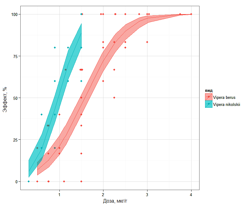
Fig. 1. "Dose-response" curves built using logistic regression and their 95 % confidence intervals for the populations with the predominance of diagnostic features of V. b. berus or V. b. nikolskii.
Further the questions if the received dependences “dose – effect” are statistically significant and how strongly contributing factors can influence their character were considered. Table 2 shows the results of the comparative statistical analysis of the four basic models in increasing their parametricity. As is customary in R, the structure of regression models was set as a “formula”, in which the dependent variable (pd – share of dead animals) is separated from the right part by the sign ~, while the predictors are separated by the sign +.
Table2. The assessment of statistical significance of the inclusion of random effects into a model
| Model | Formula | AIC | Deviance D | χ2 | P(>χ2) |
| m0 | pd ~ 1 | 587.08 | 437.84 | – | - |
| m1 | pd ~ доза | 312.58 | 161.35 | 276.49 | ≈ 0 |
| m2a | pd ~ доза + подвид | 272.14 | 118.9 | 42.45 | ≈ 0 |
| m2b | pd ~ подвид + подвид:доза – 1 | 264.17 | 108.93 | 9.97 | 0.0016 |
In the presented series the values of AIC-criterion constantly decrease that testifies of the gradual improvement of a model. The statistical significance p of including each new term (first – dose, then species) was evaluated based on the difference of residual deviances (Di-1 – Di). The latter has distribution χ2, and if it was rather high (p < 0.05), the share of variation explainable by the new term was considered reliably significant. The Fig.2 shows that the random effect is manifested as a statistically significant parallel shift of curves “dose – effect” due to the correction of an absolute term in the model m2a. Model m2b additionally takes into account the differences in the rate of effect development when increasing the dose due to correction of the coefficient of the inclination angle. The comparison of m1 и m2a tests the hypothesis of parallelism, while m1 and m2b – the hypothesis of the “equivalence” of toxic processes (Robertson et al., 2003).
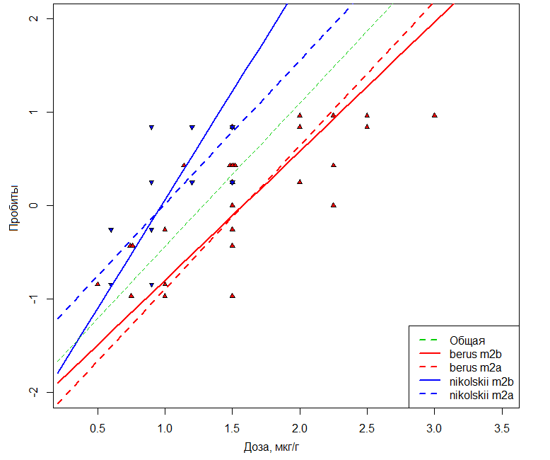
Fig. 2. Graphs of the dependence of probit values of the probability of mice death under the action of V. b. berus or V. b. nikolskii venoms. The dotted line shows the dependencies constructed under the m2a supposition that the subspecies differences are reduced to parallel shift by the magnitude of the DL50 difference. The solid lines correspond to the m2b model additionally considering the differences in the slope angle
The mixed model of an optimal structure was obtained by the method of “all possible regressions”, after carrying out the full search of combinations of random factors. Models-candidates were ranked according to the reduction of the adjusted AIC-criterion (Table 3). The relative likelihood (strength of evidence (Burnham, Anderson, 2002) of each model mmi in relation to the best model was evaluated as li = exp(-0.5 Δi), where Δi = (AICci – AICcmin). Based on that one can conclude that the model mm1 taking into account the effects of species and habitat explains the experimental results 2.2 times better than the model mm2, and it is 7×10⁶ times more proved (from the view point of probabilities ratio of corresponding hypotheses) than the model mm7 demonstrated in Fig.2.
Table3. Ranking models variants with mixed effects according to the reduction of the informational criterion Akaike AICc
| Model | Abs.term | dose | Random effects | Degrees of freedom df | Criterion AICc | Δ | ||||||
| subspecies | Habitat | sex | ||||||||||
| mm1 | -2.39 | 1.964 | + | + | 8 | 262.7 | 0 | |||||
| mm2 | -2.407 | 1.863 | + | 5 | 263.5 | 0.78 | ||||||
| mm3 | -2.576 | + | + | 7 | 266.9 | 4.16 | ||||||
| mm4 | -2.412 | 1.825 | + | + | 8 | 268.6 | 5.85 | |||||
| mm5 | -2.391 | 1.959 | + | + | + | 11 | 269.7 | 6.97 | ||||
| mm6 | -2.429 | + | + | + | 10 | 273.9 | 11.16 | |||||
| mm7 | -2.195 | 1.825 | + | 5 | 276.2 | 13.46 | ||||||
The interpretation of the model with mixed effects is based on the fact that for each level of a random factor marked with + in table 3 the system of coefficients carrying out the correction of the model with fixed parameters is selected. For example, a fixed part of the model mm1 is given by Φ-1(P) = -2.39 + 1.964·dose. If the venom of V. b.berus was used, then the term (-0.132 – 0.313·dose) was added to this equation, but if it was that of V. b. nikolskii, then (0.129 + 0.305·dose). Similarly, for the level Atkarsk of the factor habitat – specimen 2 – the term (-0.1·dose) was added, for Samara - specimen 10 – the term (+0.32·dose) and so on. And then the complete equation of regression taking into account the random parameters for the combination “probability of death by the venom of adders V. b. nikolskii, caught in Atkarsk” takes the form
Φ-1(P) = (0.129 - 2.39) + (1.964 + 0.305 – 0.1)·dose.
The series of such dependences “dose – effect” on the experimental results is given in Fig.1.
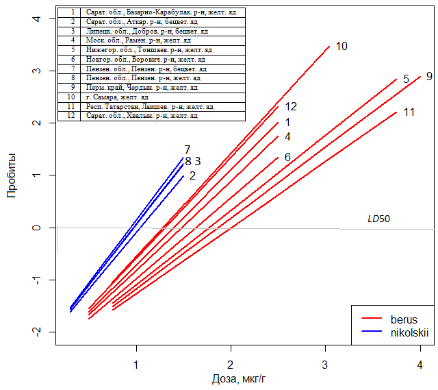
Fig. 3. «Dose-response» dependences for the venom of adders from the populations conventionally related to V. b. berus or V. b. nikolskii subspecies
The sex of experimental animals does not significantly influence the development of toxic process, and it was not included into the finally selected models.
Discussion
The analysis of patterns obtained using models mm1 allows to confirm a number of meaningful hypotheses on spatial distribution of individual populations of adders and their systematic status. In Table1 the statistically significant difference of LD50 for the subspecies of adders V. b. berus и V. b. nikolskii is shown. However, in fact, the analyzed samples were partly made in the vast zone of intergradations of the two forms, and it was possible to determine the systemic status of individual populations to a large extend arbitrary. In increasing the venom toxicity in relation to mice a geographical trend is revealed (see Fig.3) having a direction from Perm Region to Lipetsk area. It well reflects the modern ideas about the history of dispersal and hybridization of more ancient Nikolsky’s adder with the relatively young nominative form of the common adder featuring less toxic poison for mice.
The taxonomic affiliation of the forms with mixed features berus and nikolskii is to be clarified for a lot of habitats, since diagnostic features themselves of the latter form need clarification. In particular, to date the populations of V. b. nikolskii without melanists became known (Zinenko et al., 2010). Therefore, the black color of adult individuals cannot be the diagnostic feature of Nikolsky adder. Besides, its holotypes were obtained in the contact zone of V. b. berus и V. b. nikolskii (Bakiev et al., 2005; Milto, Zinenko, 2005). In connection with the fact that there is a possible prospect to reveal “clearer” populations of a forest-steppe form to the West of the typical territory of Nikolsky adder (Zinenko et al., 2010), the attention should be paid to the article 23.8 of the International code of zoological nomenclature. It indicates that the name of the species group subsequently seemed to be a hybrid must not be used as a valid name for any parent species. Therefore, if the form «nikolskii» from a new territory is re-described, its name and diagnostic features should be changed. The toxicity of the venom can be used as a new diagnostic feature.
Conclusions
- The calculation of point toxicometry indicators (LD50 of the venom of common adders for mice) by Belenky (1963) using modern versions of probit-regression failed to reveal considerable differences in final results.
- The usage of generalized models obtained by the method of maximal likelihood enables to study the toxic process over the entire range of exposure levels, to assess confidence intervals, to analyze the differences in poison power on the basis of the apparatus of statistical hypothesis testing.
- Generalized linear models with mixed effects (GLMEM) give the possibility to estimate quantitatively the influence of the complex of related random factors on the investigated processes and to suggest the changes of the reaction in different impact conditions.
- Poison toxicity can be used as a diagnostic feature when re-describing the forest-steppe form of the common adder.
References
Babich P. N. Chubenko A. V. Lapach S. N. Application of the probit-analysis in toxicology and pharmacology using Microsoft Excel program for the estimation of pharmacological activity in an alternative form of reactions registration, Sovremennye problemy toksikologii. 2003. No. 4. P. 80–88.
Bakiev A. G., Böhme W., Joger U. Vipera (Pelias) berus nikolskii Vedmederya, Grubant und Rudaeva, 1986 – Waldsteppenotter, Handbuch der Reptilien und Amphibien Europas. Band 3/IIB: Schlangen (Serpentes) III. Viperidae. Wiebelsheim: AULA-Verlag, 2005. S. 293–309.
Belen'kiy M. L. Quantitative estimation elements of the pharmacological effect. L.: Medgiz, 1963. 152 p.
Bliss C. I. The calculation of the dosage-mortality curve, Annals of Applied Biology. 1935. Vol. 22. Issue 1. P. 134–167.
Burnham K. P., Anderson D. R. Model selection and multimodel inference: a practical information-theoretic approach. New York: Springer, 2002. 448 r.
Chetverikov A. A. General linear mixed-effects models in cognitive researche, Rossiyskiy zhurnal kognitivnoy nauki. 2015. T. 2 (1). P. 41–51
Demidenko E. Mixed Models: Theory and Applications with R. 2nd ed. Wiley, 2013. 754 p.
Finney D. J. Probit Analysis. A statistical treatment of the sigmoid response curve. Cambridge: Cambridge University Press, 1947. 256 r.
Finney D. J. Probit Analysis. Cambridge: Cambridge University Press, 1971. 333 r.
Gelman A. Analysis of variance: Why it is more important than ever, The Annals of Statistics. 2005. Vol. 33. No 1. P. 1–53.
International code of zoological nomenclature. Fourth edition. M.: T-vo nauch. izdaniy KMK, 2004. 223 p.
Mastickiy S. E. Shitikov V. K. Statistical analysis and data visualization using R. M.: DMK Press, 2015. 496 p.
Milto K. D., Zinenko O. I. Distribution and Morphological Variability of Vipera berus in Eastern Europe, Herpetologia Petropolitana: Proceedings of the 12th Ordinary General Meeting of the Societas Europaea Herpetologica. St. Petersburg, 2005. P. 64–73.
Pinheiro J. C., Bates D. M. Mixed-Effects Models in S and S-PLUS. Springer, 2000. 530 p.
Robertson J. L., Savin N. E., Preisler H. K., Russell R. M. Bioassays with arthropods. Boca Raton: CRC Press, 2007. 224 p.
Zinenko O., Turcanu V., Stugariu A. Distribution and morphological variation of Vipera berus nikolskii Vedmederja, Grubant et Rudaeva, 1986 in Western Ukraine, The Republic of Moldova and Romania, Amphibia-Reptilia. 2010. Vol. 31. P. 51–67.
Acknowledgements
The authors are grateful to G.V. Yeplanova, A.V. Pavlov, M.V. Pestov, V.G. Starkov, and M.V. Ushakov for their help in collecting samples of viper venom.

 © 2011 - 2026